
Reinforcement Learning is a field of Machine Learning which aims to develop intelligences that learn through trial and error by exploring and interacting with their environment.
You may have seen exciting demos of an AI learning to play video games or robot arms learning to manipulate objects or mimic tasks.
In this post, we’ll look at a very basic approach to Reinforcement Learning which we can use to learn to play very simple games. It’s a limited approach and we’ll quickly find problems with it, but that will set us up nicely for a follow up post on how we can improve on this technique
State, Actions and Rewards
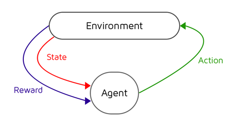
Reinforcement Learning (RL) consists of two actors: an agent (our model / algorithm), and the environment (the game we’re playing in this case). Our agent seeks to develop an optimal policy for interacting with the environment that maximises the cumulative reward over time.
Our environment is represented by a series of states. If we think of a grid with a single playing piece, we can transition states by moving our piece around the board. Each move takes us to a different possible state that the game can be in. We have several different things we can do to our piece, known as actions. We can move up, down, left, or right. Each of these actions transitions us to a new state and brings us one step closer to, or further away from, our goal state (usually a state that will win the game).
When we take an action in our game, we receive some feedback, usually in the form of a score. It’s this reward that we seek to maximise over our time playing the game.
In short, our agent interacts with our environment by choosing actions (a) to take at a particular state (s) with the intention of maximising future rewards (r) received. It’s this mapping of what action we should take at what particular state that’s the problem that we need to solve and is referred to as the policy (π), with the optimal policy being denoted as π*
The Q-Table
There are a lot of different techniques that we can use to get our model to converge on an optimal policy but in this post, we’re going to go for the one which allows us to get something up and running quickly.
Q-Learning is a technique that seeks to assess the quality of taking a given action at a given state. If we drew up a table, with all our game states as rows, and all our possible actions as columns. We could use it as a cheat sheet to keep track of the rewards we recieve for a state action pair over time. If we move left at state 1, and receive a reward of +1, we’ll write that down in our table. Over time, we’ll begin to build up a picture of the quality of every action we can take at every state, and could easily select the actions with the biggest score, or Q-value, to cheat our way to the end of the game.
But this raises two important questions, how do we update our score for each state action pair? And, how do we move around our game when we have no values in our table yet?
The Bellman Equation
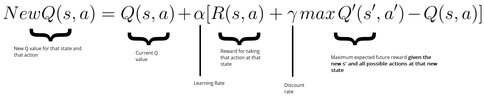
The Bellman Equation provides the foundation for assessing the quality of taking a given action at a given state. If we know the rewards at each state in the game, for example, landing on a safe tile is +1 point, and losing the game is -10 points, we can use the Bellman equation to calculate the optimal Q-value for each state action pair.
We’ll iteratively update our Q-values in our Q-table until we converge to the optimal policy, seeking to reduce the loss between our Q-value, and our optimal Q-value.
Firstly, we’ll need to take an action from our state. Then we’ll receive our reward, along with a new state. We can use this new information, along with the information of the action we took at the previous state to assess how good or bad our move was.
What if we come across a reward for a state action pair we’ve already seen? Over writing previous Q-values would lose valuable information about previous game plays. Instead, we can use a learning rate to update our Q-value. The higher the learning rate, the more quickly our agent will adopt new values and disregard previous values. With a learning rate of 1.0, our agent would simply rewrite all the old values with new values each time.
Exploration vs Exploitation
Imagine our agent is playing a game with an empty Q table. Initially, it’ll be fairly useless, so using it as a policy to follow won’t get us anywhere. In fact, when we do build up values in our Q table, we’ll want to avoid using them too early before they’ve converged. If we exploit our table too soon, we’ll get stuck at early rewards and possibly miss out on taking larger rewards that could benefit us long term.
Instead, we’ll want to strike a decaying balance between how much we want to explore the games state spaces to find new rewards, and how much we want to exploit our Q table for the correct answers. This is referred to as exploration vs exploitation.
We’ll do this with a strategy known as epsilon greedy. We’ll set an epsilon number, which represents our probability of choosing exploration vs exploitation. With epsilon set to 1.0, we have a 100% chance that we’ll explore our environment, and thus take actions entirely at random. With epsilon at 0, we’ll exploit our Q-table and select the action with the highest value. As we iterate through our training, we’ll slowly decay epsilon by gamma, a small number, that will make it less and less probable over time that we’ll explore our environment by selecting random actions.
Frozen Lake
Frozen Lake is a game where we have to navigate a 4x4 grid of tiles, each of a different surface type. S is our starting point, G is our goal point, F are frozen tiles (safe to step on) and H are holes which we can fall into and lose the game. We’ll train an agent to safely navigate from the starting tile to our goal tile using Q-Learning.
SFFF
FHFH
FFFH
HFFG
We’ll first import OpenAI’s gym library, which will give us the FrozenLake game, with a nice wrapper to be able to access actions and the state space. We’ll also require numpy and random.
import numpy as np
import random
import gym
Next we’ll start up our FrozenLake game and assign the environment to a variable we can use later on
env = gym.make("FrozenLake-v0")
In order to form our Q table, we’ll need to know the number of possible actions and states. We’ll then create an empty table, initialised with zeros at the moment, that we can later update throughout our training with our Q values, much like how we update weights in a neural network. Our Q table acts like a cheat sheet, reflecting the quality of taking that particular action, at a particular state.
action_size = env.action_space.n
state_size = env.observation_space.n

qtable = np.zeros((state_size, action_size))
print(qtable)
[[0. 0. 0. 0.]
 [0. 0. 0. 0.]
 [0. 0. 0. 0.]
 [0. 0. 0. 0.]
 [0. 0. 0. 0.]
 [0. 0. 0. 0.]
 [0. 0. 0. 0.]
 [0. 0. 0. 0.]
 [0. 0. 0. 0.]
 [0. 0. 0. 0.]
 [0. 0. 0. 0.]
 [0. 0. 0. 0.]
 [0. 0. 0. 0.]
 [0. 0. 0. 0.]
 [0. 0. 0. 0.]
 [0. 0. 0. 0.]]
Let’s set some hyperparameters…
episodes       = 10000      # Total episodes
max_steps      = 99         # Max moves per episode - stops us exploring infinitely

learning_rate  = 0.8        # Learning rate
gamma          = 0.95       # Discounting rate

epsilon        = 1.0        # Exploration vs exploitation rate
decay_rate     = 0.001      # How much we want to decay our exploration vs exploitation rate
We’ll write some helper functions that will make it easier to understand what our code is doing without getting caught up in the formulas.
Firstly, we’ll need a function that, over time, will make a gradual progression from exploration of our environment, to exploitation by utilising our Q table. We’ll use epsilon to denote our exploration vs exploitation rate, and reduce it by our decay_rate for every episode.
max_epsilon is the largest our epsilon can be and represents a full 100% chance we’ll explore our environment. Conversely, min_epsilon represents a 100% chance that we’ll exploit our Q table for the correct answers.
def reduce_epsilon(episode, min_epsilon=0.01, max_epsilon=1.0, decay_rate=0.001):
    return min_epsilon + (max_epsilon - min_epsilon) * np.exp(-decay_rate * episode)
Epsilon will be used in selecting wether we want to explore our environment, which we’ll do by selecting an action at random, or wether we want to exploit our learned Q-table, which we can do by selecting the action with the highest Q value.
Since this is fairly simply logic, we can code this into another helper function which will help simplify our code…
Here we take in some information like our epsilon, our qtable, state and the env (environment) and generate a random number. If our number is larger than epsilon, we’ll choose to exploit our Q-table by selecting the action with the highest Q-value. If our number is lower than epsilon, we’ll explore our environment further by selecting a random action from our action space.
def select_action(epsilon, qtable, state, env):
    x = random.uniform(0,1)

    if x > epsilon:
        # Exploitation
        return np.argmax(qtable[state,:])
    else:
        # Exploration
        return env.action_space.sample()
Lastly, we’ll need a function to update the values in our Q-table based upon the Bellman equation given our previous state, action taken, reward, and new state…
def update_qtable(qtable, state, action, reward, new_state, learning_rate, gamma):
    # Update Q(s,a):= Q(s,a) + lr [R(s,a) + gamma * max Q(s',a') - Q(s,a)]
    # qtable[new_state,:] : all the actions we can take from new state

    qtable[state, action] = qtable[state, action] + learning_rate * (reward + gamma * np.max(qtable[new_state, :]) - qtable[state, action])
    return qtable
Training our Q-Table
Next up is the bulk of our code. This is where we’ll put the pieces together, train our agent, and populate our Q-table.
For every episode in our total number of episodes, we’ll firstly reset our environment and a few variables which will keep track of game play for that particular run. For each step, we’ll use our select_action() function to choose an action, either at random (exploration) or from our Q-table (exploitation). This rate will gradually ramp towards more and more exploitation over time as we build up our Q-table.
We’ll then take our action and observe the reward and new state returned, which we’ll use to update our Q-table. Finally, we’ll we’ll set our state to be the new_state that we received by taking an action, reduce epsilon to lean slightly more towards exploitation, add our reward to a list so that we can keep track of how we’re improving over time, and start the cycle over again until we reach some terminal state in our game (we fall into a hole, or win the game).
rewards = []

for episode in range(episodes):
    # Reset the environment
    state = env.reset()
    step = 0
    done = False
    total_rewards = 0

    for step in range(max_steps):
        # Use epsilon to pick an action, either at random, or from our q-table
        action = select_action(epsilon, qtable, state, env)

        # Take the action and observe the new state and reward
        new_state, reward, done, info = env.step(action)

        # Update our Q-table to take note of how valuable the action according to the reward we got
        qtable = update_qtable(qtable, state, action, reward, new_state, learning_rate, gamma)

        # Set state to the new state we received (where we moved to)
        state = new_state

        total_rewards += reward

        # If the game is over, exit the loop, back to a new training loop
        if done == True:
            break

        epsilon = reduce_epsilon(episode)

    rewards.append(total_rewards)

print("Score over time: " +  str(sum(rewards)/total_episodes))
print(qtable)
Playing the Game
Once we’ve populated our Q-table, we can exploit it to play the game successfully. As we’re simply following our Q-table, we no longer have to deal with updating our table, or dealing with our exploration vs exploitation trade off. We can simply just follow the policy of selecting the highest value at a given state. With a well trained Q-table, our values should closely reflect the maximum expected reward over time by taking that particular action at that particular state.
env.reset()

for episode in range(5):
    state = env.reset()
    step = 0
    done = False
    print("Playing Round #", episode)

    for step in range(max_steps):
        # Select the action with the highest reward
        action = np.argmax(qtable[state,:])

        # Return our new state and reward
        new_state, reward, done, info = env.step(action)

        if done:
            # If the game is finished, we'll print our environment to see if we fell into a hole, or ended on our goal tile
            env.render()

            # We print the number of steps it took.
            print("Steps taken:", step)
            break

        state = new_state

env.close()
Summary
And there we have it! We successfully trained a model to learn play the Frozen Lake game by exploring the environment itself, and learning through trial and error.
But what happens when we want to play a more complex game with millions of possible states? Unfortunately, as your state space grows, you very quickly out grow the feasibility of using a Q-table. It would take millions of iterations to even begin to explore all the possible state spaces and build up an accurate Q-table.
Instead of creating a cheat sheet that we can look up every possible value for every possible action in every possible state, what if we could just simplify by having a function that approximates the Q-value for a given state action pair?
If you have read previous posts, you may be familiar with one tool that we can use for function approximation; the neural network.
In a future post we’ll look at how we can improve on our reinforcement learning agent by using neural networks to apply our techniques to larger state spaces and more complex games with Deep Q-Learning.