
In the past few posts, I’ve taken a dive into how neural networks work. We even built a neural net that could learn to recognise handwriting by breaking it down into a huge array of the pixels in the image, and representing the colour of the pixel as a value from 0-1.
Our last model got 96% accuracy, but it turns out we can do even better with a different type of neural network that is especially good at images; the convolutional neural network.
In this post we’ll explore the concept of convolutional neural networks, how they work, what makes them good at dealing with images and build our own using Tensorflow.
What is convolution?
Convolution simply means combining two things to form a third thing, which is a modified version of one of the first things. Let’s look at how it works in detecting edges in an image…
Let’s take a small sample of our larger image. We’ll zoom in on a 5x5 grid of the top corner of our image. Our image will be our first input, which we’ll need to convolve with some other input, to create our output. That second input will be called our filter. A filter is simply a smaller grid of weights, and we’ll slide this over our 5x5 image sample like in the gif above.
You can see the weights written in red. At each step, we’ll take each number in our 3x3 window of our image and multiply it by the corresponding weight in our filter cell. So in the top left hand corner, our value is 1, and our filter value is 1, therefore, 1x1 will be 1, and we’ll add this to the next value where our image value is 1 but our filter value is 0.
We’ll repeat the process until we have a total for the values within our filter. This ends up giving us a total of 4. We’ll write this in our output, and slide our filter one cell over to the right and repeat to get the next value. Once we reach the end of the row, we’ll slide one cell down and back to the left and repeat the process. Repeating this for a 5x5 grid will give us a 3x3 output.
The different values in our filter enhance differences in the image. We can use a filter to detect edges for example by having values in the first and third columns of our 3x3 grid that result in a negative total, and values in the middle column that results in a positive total when passed over an edge. This would result in an output something like this, showing a dark to light to dark edge…
0,1,0
0,1,0
0,1,0
That’s really all there is to it; filters give us a convenient way to find certain features in an image by their light/dark difference represented numerically. But which filters to use? Well this is something that we will let our neural network learn. During training, it will learn the right features for the job.
Padding
When we slide our filter over our image, we’ll only touch on the corner pixels once, but the middle pixels end up in lots of our windows. This is a problem as this is giving more importance to the middle pixels than the outer ones. We want every pixel to have an even influence in our calculations. Also, our output is now 3x3, so we’ve lost some size. How do we solve these issues?
The answer is padding. We’ll add an extra border of pixels around our image. This means that when we slide over our image with our filter, we not only are able to reach our original edges the same amount of times as we reach the middle pixels, but that our output ends up being the same size as our input. When the output is the same as the input size, this is called same padding. When we add no padding, we call this valid padding.
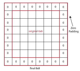
Padding is another hyperparameter that we can tune for our network. It doesn’t just have to be one pixel we pad with; a 5x5 image will require a padding of 2 to give a 5x5 output.
Strides
In our example we took a 5x5 grid and slid our filter over one cell at a time. The distance we move our filter is called a stride. In our example we had a stride of one; moving one cell at a time. Setting the stride to 2 would jump our filter two cells across, and when we reached the end of a row, we would jump two rows down.
Dealing with RGB images
As any RGB images we input will have three dimensions (one each for red, green and blue), our images are no longer 5x5, but they are 5x5x3. To deal with this, we’ll do the same with our filters, having a filter for each channel.This is why you often see convolutional neural nets drawn with cubes or three dimensional objects instead of squares. The cube simply represents the channels of our image, or that our image is three dimensional (in the sense that colour is our third dimension). Using these 3d filters, we can also start to recognise features in different colours by applying different filters to different colour channels.
Pooling
Pooling is a technique that can be used to speed up our network and reduce computation.
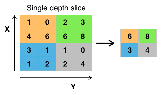
We’ll take our input and split it into different regions (in this example, we’re taking a filter size of 2x2 and a stride of 2), and we’ll simply take the largest number in the region. This is called max pooling, as we’re taking the maximum value.
Max values usually represent that a feature has been detected so we can keep this, and move it to our new output. Our filter size and stride are also tunable hyperparameters here, other than this, we have no parameters to learn for max pooling, it’s just a fixed computation which we apply through each channel.
Forward Propagation
The weights for our 3x3x3 filters will play the role of standard weights in forward propagation of our network. We’ll add a bias to give us a total of 28 weights (3x3x3 = 27 + 1 = 28) and apply an activation function as normal. Let’s work through an example
Let’s assume that we have a small input image of 39x39 pixels, with 3 channels (RGB), giving us a 39x39x3 input into our convolutional neural net.
In our first layer, we’ll use a set of 3x3 filters to pass over our image. We’ll use a stride of 1 and no padding. We’ll have 10 filters in our first layer.
This means our activations for our first layer will be 37x37x10. The height and width are explained by the moves we can make with a stride of one, we lose a little bit of size because we cant overlap our filter over the edges. Our depth comes from the fact this this activation represents a stack of learned filters and since we learned 10 filters, our output for this layer will be 10 filters deep.
Our formula for our output of a layer looks like this…
# nh = height of input in pixels (39)
# p  = padding
# f  = filter size (3)
# s  = stride size (1)

((nh + (2 * p) - f) / s) + 1 # This + 1 is adding our bias
We can also change nh for nw to get the width.
In our second layer, we’ll use a 5x5 filter, with a stride of 2, and no padding to apply 20 filters. We can follow our formula above to get our output size…
nh = 37
p  = 0
f  = 5
s  = 2

((nh + (2 * p) - f) / s) + 1

or

((37 + (2 * 0) - 5) / 2) + 1
This gives us an output of 17x17x20. Because we used a bigger stride this time, our size shrank quite dramatically and our depth grew because we applied more filters.
Let’s do one more layer. We’ll input our 17x17x20 and use a 5x5 filter, with a stride of 2 to apply 40 filters. Using the same formula, we get a 7x7x40 output.
After we perform a few layers of convolution, we’ll take our output and flatten it into a single long array. A 7x7x40 array will unroll into a 1960x1 list of values which we can then feed into a few layers of standard neurons with a softmax function to get our final output.
Putting it all together
Traditionally, we’ll intersperse our pooling operations with our convolutional layers and then feed the whole thing to a few fully connected layers, before using softmax to give our final output. Our pooling operation isn’t really counted as a layer as it doesn’t have any weights to learn, so we’ll often group a convolutional and a pooling operation as part of the same layer.
| Layer | Size | Settings |
|---|---|---|
| Input | 32x32x3 | f=5, s=1 |
| Conv1 | 28x28x8 | |
| MaxPool | 14x14x8 | f=2, s=2 |
| Conv2 | 10x10x16 | f=5, s=1 |
| MaxPool | 5x5x16 | f=2, s=2 |
| Full | 120x1 | |
| Full | 84x1 | |
| Softmax | 10x1 |
Note we’re outputting to 10 neurons, so in this example we’re assuming you’d want to classify something as one of 10 classes, for example, our 0-9 hand written number recognition task.
Also notice the size of our data as it passes through our network. It stays relatively small. If we’d have just unrolled our 32x32x3 image into one long vector, and fed it to even more neurons, which get fed to even more neurons, the amount of weights in our network would be huge. We’d face our exponential complexity problem again we discussed a few posts back in Neural Networks from Scratch.
Instead, the only parameters we learn are those of our relatively small 3x3 or 5x5 filters, and while we may have a lot of them, it doesn’t get out of hand anywhere near as quickly as if we treated each pixel as a neuron.
Summary
Convolutional networks allow us to learn filters, which can then be reused as we pass them across the network looking for interesting features. As we combine these features together we can detect more high level features and combine the result to get even more higher level information about the features. Detected edges, when combined, can tell us where a curve is, and detected curves, when combined, can tell us where a nose or an eye is, and detected noses and eyes when combined can tell us the presence of a face.