
In this post we’ll take a dive into the maths behind neural networks and how they work by building our own neural network from scratch using Python.
WTF is a neural net?
Our brains are full of billions and billions of neurons stacked together. They look a little something like this…
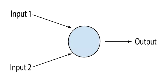
At their core, they’re just a cell that takes in some very basic electric signals, and decides wether to fire a signal to the next neuron or not based on the signals it receives. A single neuron on it’s own isn’t very useful, but when we start stacking lots of neurons together, and let each of them handle a tiny bit of information in the form of an electrical impulse, we get a brain, and it turns out brains are actually pretty good at complex stuff.
In the 50s a bunch of researchers decided to take inspiration from the way the brain works and create an artificial neuron (this is what is in the diagram) that would take in a set of numbers, perform some kind of function (like adding them together for example) and then pass the result to the next neuron. We could even stack lots of neurons together to make a neural network just like the brain! This was a great idea, but in the 50’s, we didn’t have the computing power or the amount of data needed to make it work.
Fast forward to today and neural nets are the new hotness of 2016/17 and sit at the heart of Netflix’s recommendation systems and Tesla’s autopilot.
Supervised learning
Neural networks are a supervised learning problem. This means they rely on supervision to learn, we have to actively train them by giving them a bunch of correctly labelled answers and letting it work out how we got to them.
Imagine your job was to replicate a recipe for a cake. You likely wouldn’t know where to begin, but if you had a correct list of ingredients and the final cake to reference, you would just need to keep making cakes and tweaking your recipe until you were able to match the look and taste of your reference cake.
Building a neural network
We’ll import our dependencies and fix our seed so that our random numbers are the same every time we run our code
import numpy as np
np.random.seed(1)
Neural networks have two stages that we need to code; forward propagation (which is just passing data through our network to make a prediction) and back propagation (which is the art of calculating how wrong our prediction was, and adjusting the weights to move us a little closer to a more correct prediction).
We’ll start by creating a class for our neural net and initialising all our weights with a random starting point. We’ll save these in our instance for later use…
class NeuralNetwork():
    def __init__(self, input_layer_size, hidden_layer_size, hidden_layer_2_size, output_layer_size):
        # Initialise the weights for inbetween each layer
        self.w1 = np.random.randn(input_layer_size, hidden_layer_size)
        self.w2 = np.random.randn(hidden_layer_size, hidden_layer_2_size)
        self.w3 = np.random.randn(hidden_layer_2_size, output_layer_size)
We’ll add a few helper functions to our class to calculate the sigmoid of a given number, and the sigmoid derivative. These will come in handy later…
    def __sigmoid(self, x):
        return 1 / (1 + np.exp(-x))

    def __sigmoid_prime(self, x):
        # Calculates the derivative of our sigmoid function
        return np.exp(-x) / ((1 + np.exp(-x)) ** 2)
Forward Propagation
We’ll multiply the inputs by the weights for the first layer, and apply a sigmoid activation function. Once we have this, we’ll repeat the process and multiply our result by the weights for the second layer, and apply our activation function. We’ll rinse and repeat until we get to the end of our network.
    def forward_propagation(self, inputs):
        # Z's are pre activation function, A's are post activation function

        # Feed inputs to first hidden layer
        self.z2 = np.dot(inputs, self.w1)
        self.a2 = self.__sigmoid(self.z2)

        # Feed first hidden layer to second hidden layer
        self.z3 = np.dot(self.a2, self.w2)
        self.a3 = self.__sigmoid(self.z3)

        # Feed second hidden layer to output to generate prediction
        self.z4 = np.dot(self.a3, self.w3)
        prediction = self.__sigmoid(self.z4)

        return prediction
Cost Function
Once we have our prediction, we now need to work out how bad we were. We can use a cost function to quantify exactly how bad our prediction was.
One method of doing this is to take all the errors, square them, and get the average. This is called the Mean Squared Error (MSE). The goal of training our neural net then becomes to try to minimise this cost. The lower our error (given to us by the cost function), the better our predictions will be.
Let’s add a helper function to our class to calculate our cost…
    def __compute_cost(self, prediction, actual):
        # Compute the Mean Squared Error of our inputs
        # This gives us an overall averaged cost of how wrong our prediction was
        return np.sum(0.5 * (actual - prediction) ** 2)
Backpropagation
The weights in our neural net are our variables we can tweak that allows our network to generate good predictions. We want to find the best set of weights that result in the closest predictions. We work backwards from our prediction, back to our inputs to tweak these weights. This backwards pass through our network is called backpropagation or backprop.
Wait. Why can’t we just check all of the possible weights? Well for a start all the weights need to work together, and as we add more, the difficulty grows exponentially. Imagine cracking a 4 digit pin number, there are 10^4 possibilities, that’s 10,000 different pin numbers. If we just add one more digit to our pin number, the possibilities jump to 100,000. That means our total combinations just shot up by 90,000! A six digit pin has 1,000,000 combinations! Going from 5 to 6 digits results in an extra 900,000 combinations! As we add more weights, our complexity and difficulty in brute forcing this grows exponentially.
So how can we adjust our weights to reduce our cost function? What if we knew which direction to tweak our weights would result in reducing the cost function? Well we could test the cost function of each side of our prediction to see which side is smaller, but that would be time intensive.
Maths to the rescue! We can use the partial derivative which says “What is the rate of change of our cost function (J) with respect to W?”
Calculating the partial derivative will give us a positive value for our cost increasing, and a negative value for it decreasing.
    def backpropagation(self, inputs, labels, predictions):
        delta4 = np.multiply(-(labels - predictions), self.__sigmoid_prime(self.z4))
        dJdW3  = np.dot(self.a3.T, delta4)

        delta3 = np.dot(delta4, self.w3.T) * self.__sigmoid_prime(self.z3)
        dJdW2  = np.dot(self.a2.T, delta3)

        delta2 = np.dot(delta3, self.w2.T) * self.__sigmoid_prime(self.z2)
        dJdW1  = np.dot(inputs.T, delta2)

        return dJdW1, dJdW2, dJdW3
We’ll iteratively take tiny steps downhill by calculating our cost, seeing which way to move, and shaving a tiny preset number which is called our learning rate, off our weights, and then running the cost function again, using our derivative to see which way to move, and taking another tiny step. The learning rate can be thought of as the size of the step we’re taking. Take too bigger step and we might miss the lowest error and bounce back up. Take too smaller step and our network will take forever to train.
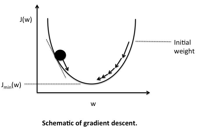
We’ll iterate with tiny steps until our error stops reducing and lands in lowest point of error, or local minima. This process is called gradient descent and it is everywhere in machine learning.
Training
Once we have our gradients, we’ll need to update our network to take a small step towards reducing our cost. We’ll do this multiple times by exposing our dataset to our neural network for 5000 iterations, called epochs in machine learning.
    def train(self, input_data, labels, epochs, learning_rate):
        for iteration in range(epochs):

            # Step 1. Forward prop to get our predictions...
            predictions = self.forward_propagation(input_data)

            # Step 2. We'll print the cost to see how well we did
            print("Current cost:", self.__compute_cost(predictions, labels))

            # Step 3. Backprop to get our gradients (with which we'll update our weights)
            dJdW1, dJdW2, dJdW3 = self.backpropagation(input_data, labels, predictions)

            # Step 4. Update our weights
            # If we add our dJdW (our gradient), we'll increase our cost, and if we subtract it, we'll reduce it
            # We'll set our weights to themselves, minus a tiny amount in the direction of our gradient
            # (this is where we use a learning rate to take a tiny amount of the gradient)

            self.w1 = self.w1 - (learning_rate * dJdW1)
            self.w2 = self.w2 - (learning_rate * dJdW2)
            self.w3 = self.w3 - (learning_rate * dJdW3)
Putting it all together
Let’s create a dataset and its corresponding correct labels
input_data = np.array([[0,0,1], [1,1,1], [1,0,1], [0,1,1]])
labels     = np.array([[0,1,1,0]]).T
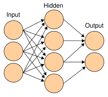
We’ll initialise a new neural net with 3 input nodes (our data is an array with 3 elements, so each one needs its own input node), 4 nodes in the first hidden layer, 5 in the second hidden layer, and 1 output…
net = NeuralNetwork(3,4,5,1)
net.train(data, labels, 5000, 0.1)
Running our code we can see how our cost decreases over time…
Cost at epoch 0: 0.688239103472
Cost at epoch 1000: 0.0192991528354
Cost at epoch 2000: 0.00398719767284
Cost at epoch 3000: 0.00202819194556
Cost at epoch 4000: 0.00132494673741
Let’s see how well our network learned to predict our test set. We can just run net.forward_propagation(data) to predict new data on our trained network…
print("Predictions...\n", net.forward_propagation(input_data))
print("Actual...\n", labels)

[[ 0.02039406]
 [ 0.96795662]
 [ 0.97199464]
 [ 0.02758648]]
[[0]
 [1]
 [1]
 [0]]
Not bad!