Python has made itself the default programming language for data science and machine learning. It’s well documented, simple to use and fun to work with.
But let’s have a look at what happens when we try to add two lists together…
list = [1,2,3]
list + list

[1,2,3,1,2,3]
Not what we expected. Lists can’t perform element wise calculations. In fact, it turns out lists in Python have some big limitations which we’ll need to solve if we want to do the kind of heavy maths needed for machine learning.
Enter Numpy. Numpy is a library for Python which adds support for large multidimensional arrays, matrices, and high level mathematical operations on these new datatypes. It’s fairly intuitive but let’s take a look at some examples…
Once we’ve imported the library, we can create a numpy array by passing in a regular Python list…
import numpy as np

list = [1,2,3]
np_array = np.array(list)

array([1,2,3])
You’ll see it’s just like a regular list, but wrapped in this array() object. Now let’s revisit our first example…
np_array + np_array

array([2,4,6])
Something to note; arrays can only contain a single data type. If we were to put a string as an element, even a single element, the entire array would be converted to strings. The same goes for floats etc. Numpy expects uniformity in our data types.
Onto some more features; we can create a random array using numpy’s random function, and passing in the dimensions of our array.
a = np.random.rand(3,3)

array([[ 0.63294935,  0.18020465,  0.95212327],
       [ 0.98974435,  0.35659871,  0.86290932],
       [ 0.46544616,  0.51164278,  0.17143704]])
We can check the shape of our array with the np.shape(a) method or just by calling .shape on an existing array…
a.shape

(3,3)
The values returned are the dimensions, starting with the 0th dimension. Most of the time, this will be (rows, columns), although Numpy supports higher dimensional arrays, so it’s entirely possible to have a shape of (5,5,5,5,5,5,5) or higher, which can be a little confusing to think about.
Accessing attributes is just the same as a list, including the use of the colon to denote all entries in that dimension…
a = np.array([[1,2,3],[4,5,6]])
a[0][1]

2
Let’s use the colon to select some ranges. Let’s try all rows, and the middle column (from column 1, up to, but not including, column 2)…
a[:, 1:2]

array([[2],
       [5]])
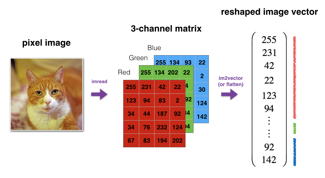
One common operation in machine learning is reshaping arrays. We’ll look at a common example; flattening an image into a single array. We’ll start with an image measuring 28 pixels by 28 pixels, and having a depth of 3 channels (representing the red, green, and blue channels in a colour image)…

image = np.random.rand(28,28,3)

length  = image.shape[0]
height  = image.shape[1]
depth   = image.shape[2]

flat_image = image.reshape(length * height * depth, 1)
flat_image.shape

(784, 3)
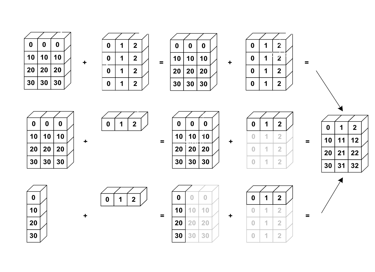
When we have two matrices or arrays of different sizes, for example a 3x3 and a 1x3, numpy will duplicate the smaller array to match the size of the other array. This is called broadcasting and will happen on most element wise operations on matrices of different sizes.
It’s probably better illustrated rather than coded. You can see how the smaller arrays are copied in grey to make up the empty space and create a compatible matrix…

Another vital operation that is used everywhere in machine learning is the dot product. The dot product is the summation of an element wise multiplication of two matrices. The dot product can be called using np.dot(a, b) where a and b are two matrices of the same size. For arrays of one dimension, the dot product will be a number, but for multidimensional arrays, the result will be a matrix of the same size as the input size…
a = np.random.rand(3,3)
b = np.random.rand(3,3)

np.dot(a, b)

array([[ 0.35544886,  0.43097739,  0.38872774],
       [ 0.73062091,  0.67305096,  0.55726258],
       [ 0.43227186,  0.54603886,  0.46658088]])
